7.3 Sentiment Analysis using VADER
Another type of sentiment-analysis we can use is known as VADER Hutto & Gilbert (2014) (Valence Aware Dictionary and sEntiment Reasoner) which is a sentiment dictionary specifically made for sentiment in social media. Also, where most dictionaries tend to depend on a single coder classifying the terms, VADER uses multiple coders in order to arrive at a dictionary. So how well does it work? Let us test this again this the airline data we had before. First, we re-load this data back into R. Then, we separate the text and select 1000 tweets to work with:
urlfile = "https://raw.githubusercontent.com/SCJBruinsma/qta-files/master/Tweets.csv"
tweets <- read.csv(url(urlfile))
tweets <- tweets[sample(nrow(tweets), 1000), ]

text <- tweets$text
We then apply VADER to our tweets. Note that the vader package has just two available commands: either to measure values for a single string, or to measure values for a dataframe. Here we will use the latter:
VADER then provides us with a dataframe consisting of seven different variables. The first contains the text, the second the “word_scores” which is a string containing an ordered list with the scores for each of the words in the text, the third the “compound” which is the sum of all the valence scores in the document, and “pos”, “neg” and “neu” refer to the positive, negative and neutral content specifically. In addition, there is an additional count for the occurrence of the word “but”, as this often complicates the calculation of any type of sentiment.
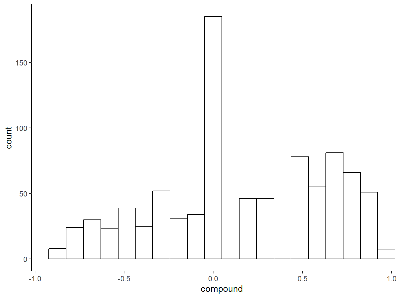
To get a better idea of the output, we can look at the distribution of the scores:
library(ggplot2)

ggplot(data = results_vader,
       aes(x=compound)
       ) +
geom_histogram(bins = 20,
               color="black",
               fill="white") +
theme_classic()
As we can see, there are quite a lot of neutral scores. If we look at the scores, tweets such as “@JetBlue Counting on your flight 989 to get to DC!” does not have any apparent sentiment, and seem to be quite often occurring, which most likely explains our results here.